- Instructions
- How and what to submit?
- Late submissions
- What is the required level of detail?
- Collaboration policy
- 1. Color Alignment
- 1.1 Synthetic ("manufactured") offsets
- Problem 1 (15 points)
- Problem 2 (20 points)
- 1.2 Real data
- Problem 3 (15 points)
- Bonus Problem (10 points)
- 2. Demosaicing
- 2.1 Linear Interpolation
- Problem 5 (20 points)
- 2.2 Freeman method
- Problem 6 (30 points)
A1: Seeing the Color
Instructions
Note that this web version (manually) mirrors the PDF and is an experimental feature. Should there be discrepancies stick to the PDF handout. HW1 is a set of relatively simple exercises that should take a few hours at most. Take the opportunity to make sure the software setup is ready and get some familiarity with image processing.
How and what to submit?
Please submit your solutions electronically via Canvas. Please submit your solution (Python code and the documentation of the experiments you are asked to run, including figures) in a Jupyter notebook file. Rename the notebook firstname-lastname-ps1.ipynb.
Late submissions
There will be a penalty of 25 points for any solution submitted within 48 hours past the deadline. No submissions will be accepted past then. Please email instructors for special circumstances.
What is the required level of detail?
When asked to derive something, please clearly state the assumptions, if any, and strive for balance: justify any non-obvious steps, but try to avoid superfluous explanations. When asked to plot something, please include in the ipynb file the figure as well as the code used to plot it. If multiple entities appear on a plot, make sure that they are clearly distinguishable (by color or style of lines and markers) and references in a legend or in a caption. When asked to provide a brief explanation or description, try to make your answers concise, but do not omit anything you believe is important. If there is a mathematical answer, provide is precisely (and accompany by only succinct words, if appropriate).
When submitting code (in Jupyter notebook), please make sure it's reasonably documented, runs and produces all the requested results. If discussion is required/warranted, you can include it either directly in the notebook (you may want to use the markdown style for that) or in the PDF writeup. Please make sure to submit a notebook that has been run with all the outputs generated.
Collaboration policy
Collaboration is allowed and encouraged, as long as you (1) write your own solution entirely on your own, (2) specify names of student(s) you collaborated with in your writeup.
1. Color Alignment
The Russian photographer Sergei Mikhailovich Prokudin-Gorskii (1863-1944) dreamed of producing color photographs, though the technology for color photography did not yet exist. He conducted photographic surveys of the Russian Empire using red, blue and green color filters to take photographs, with the camera moving slightly between shots. This leads to three images (a "triptych") of the same scene with small offsets between them (Figure 1)-- there was no way to combine these images automatically in Prokudin-Gorskii's day (instead, he painstakingly aligned them by hand), but we will develop a simple technique for aligning the images and producing the color photos he had tried to make.
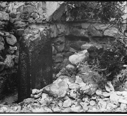

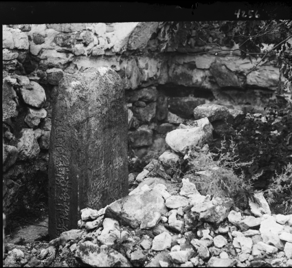
Fig 1: Red, green and blue parts of a tryptich. Note that the camera visibly moved between each shot
Specifically, we will implement an automatic procedure for taking the red, green and blue filter images and combining them into an RGB color image.
1.1 Synthetic ("manufactured") offsets
The red, green, and blue components of an image are called "channels". Due to camera motion between shots, the color channels are misaligned. We will start with a simple synthetic example to simulate this effect. We will take a regular RGB image, shift its color channels around so they become misaligned (using a random shift for both the horizontal and the vertical directions for R and B relative to G which stays in place). Then, we need to shift the channels so that they align again, finding the optimal displacement. We need to pick one of the channels as the "canonical" image, then align the other two channels to it according to a metric (measure of alignment quality). More precisely, assuming we use the green channel as the "anchor" to which we align the red and blue channels and , let be the measure of discrepancy between two single-channel images; we are trying to find
where is the set of transformations under consideration. In our case is the set of shifts of up to pixels (horizontally and/or vertically).
We can solve Eqn 1 by an exhaustive search over a window of possible displacements to align the red channel and the blue channel to the green channel. We need a metric to compare the two images as we shift color channels to align, and will implement a simple sum-of-squared-differences (SSD) metric (you are welcome to try other metrics as well).
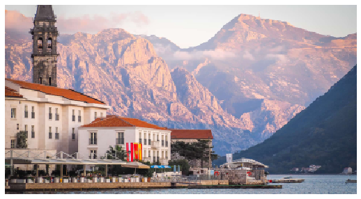
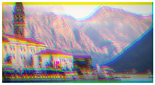
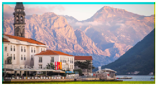
Fig 2: Original image, synthesized misaligned image, reconstructed image. You should see something similar, although not exactly the same due to random shifts.
For vectors define
Problem 1 (15 points)
Implement the image-shifting routines shift_image_y and shift_image_x. Pay attention to the axis convention and how you pad the color channels. numpy.roll may be useful here.
Load the provided image test-image.png. This is an image without misaligned color. Extract the color channels, and shift them. For this synthetic example, limit the random shifts to pixels.
Display the original image; the "naively stacked" image where you simply superimpose the shifted color channels; and the image reconstructed by inverting the shifts in the color channels using the known (ground truth) shift values. You should see something similar to images in Figure 2.
Problem 2 (20 points)
Implement get_optimal_shift that returns a tuple (dy, dx) which will be applied on misaligned color channel to correct the shifting. Use the SSD metric.
Apply this on the synthetically misaligned example we created just now. In this case we can limit the range of max_shift to pixels.
1.2 Real data
Next we will use the code you developed in the previous section on two real "triptychs" of Prokudin (one of which is seen in Figure 1).
Problem 3 (15 points)
Use the code you wrote for the synthetic example, for each triptich, display the results with the naive stacking, and the result with your optimized alignment. A code snippet in the provided starter notebook shows you how to load the three channels from separate files and display the stacked result as a color image.
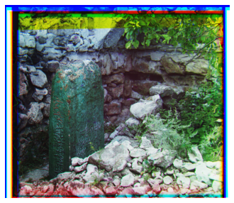
Fig 3: Aligned Prokudin-Gorskii image obtained from the 3 channel images in Fig 1.
Bonus Problem (10 points)
Pick any additional image triptych(s) from the Prokudin-Gorskii Collection and align the color channels. You wll need to crop the individual color channels by hand, using a tool (we recommend IrfanView).
Note: you may have to downsample the images to get good results at a reasonable speed with the simple technique we have described in this problem, as the raw images are rather large. Play around with image scale and offsets (for larger images the window will not work) as well as cropping the dark regions around the image for best visual effect.
2. Demosaicing
Problem 1 introduced the idea of color channel alignment for old photographs, but there is also a modern "color alignment" problem that must be solved whenever a digital picture is taken -- demosaicing.
The raw image that is captured by a real digital camera is actually a single-channel picture taken through a color filter array (CFA) that disperse the red, green and blue pixels according to some pattern. Figure 4 has a standard "RGGB" Bayer pattern we will use in this problem; you can read up for more information Note here that the green pixels are sampled more frequently than red or blue.
Our goal will be take a single-channel "Bayer image" (see Figure 6 left ) and "demosaic" it into a proper RGB image.
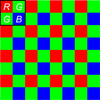
Fig 4: RGGB Bayer pattern
2.1 Linear Interpolation
We will start with a linear interpolation approach to demosaicking. The simplest possible solution to this task would be top loop through the mosaic, placing the correct value into each channel depending on the row and column based on the pattern in Figure 6. However, this approach would be prohibitively slow on large images, and so we will take a faster approach with convolution.
In class we will be discussing image filters, a pattern convolved with an image to produce a desired effect (for example, the box filter is a commonly-used low-pass filter which blurs an image). Figure 5 gives you a hint on how to design filters for each color channel.
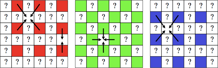
Fig 5: Demosaicking through linear interpolation.
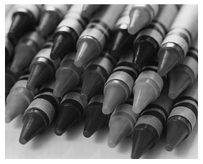
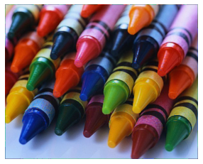
Fig 6: The raw Bayer pattern mosaic (left) which appears as a graylevel image. The RGB image once the left image has been properly separated into color channels (right).
Problem 5 (20 points)
Using the provided single-channel mosaic image crayons.bmp, apply naive per-channel interpolation and display the resulting color image next to the mosaic. You should see results similar to Fig 6. If you zoom in, you will notice some artifacts (little color splotches/speckles that clearly are a result of noisy interpolation).
2.2 Freeman method
In 1985 Bill Freeman proposed an improvement to the above approach by noting that there are twice as many samples as and . This approach starts by doing a linear interpolation as in 2.1, then keeping the channel fixed but modifying the and channels.
First, this approach computes the difference images and between the respective (naively) interpolated channels. Mosaicing artifacts tend to show up as small "splotches" in these images. To eliminate the "splotches", apply median filtering (e.g. scipy.signal.medfilt2d, or your own implementation) to the and images. Finally, create the modified and channels by adding the G channel to the respective difference images.
Problem 6 (30 points)
Implement Freeman method, play around with the size of the median filter and compare the output of this method to the original image -- is the Freeman method successful on this image? What kinds of artifacts does it erase or introduce? Display the color image with Freeman's demosaicing, and explain how you chose the filter size, and what the effects of making the filter size larger seems to be. Hint: to make the corrective interpolation work as intended, it may be useful to bring the color channels to the same mean value prior to subtractions (by removing the mean for each color channel); you need to remember to add it back before displaying the final color image.
Made with ❤ by Yours Truly.